Understanding NISQ: The Bridge to True Quantum Computing
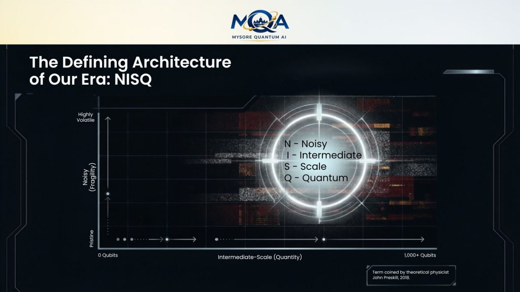
If you’ve been following quantum computing news lately, you’ve likely run into the acronym NISQ. Coined by theoretical physicist John Preskill in 2018, it stands for Noisy Intermediate-Scale Quantum.
To understand what it means, we have to look at where quantum computing is right now: a fascinating, transitional era where our hardware is incredibly powerful, yet incredibly fragile.
Let’s break down exactly what the acronym means, why it matters, and what we can actually do with it.
Breaking Down the Acronym
NISQ stands for:
N = Noisy
I = Intermediate
S = Scale
Q = Quantum
To understand NISQ, we just need to look at its two components: Intermediate-Scale and Noisy.
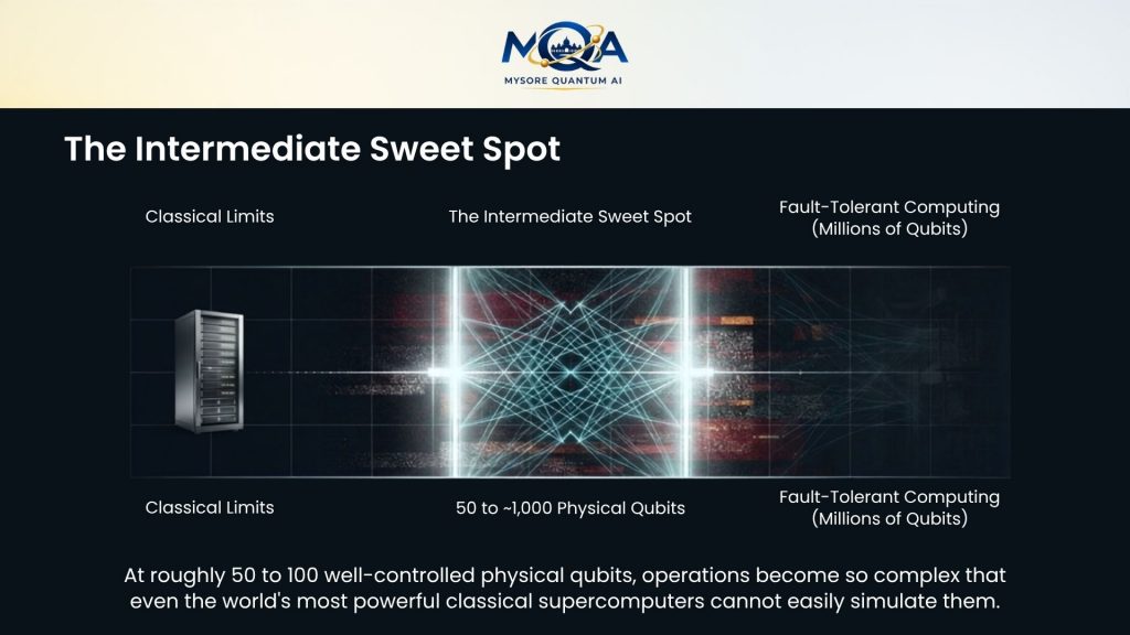
a. Intermediate-Scale (The Size)
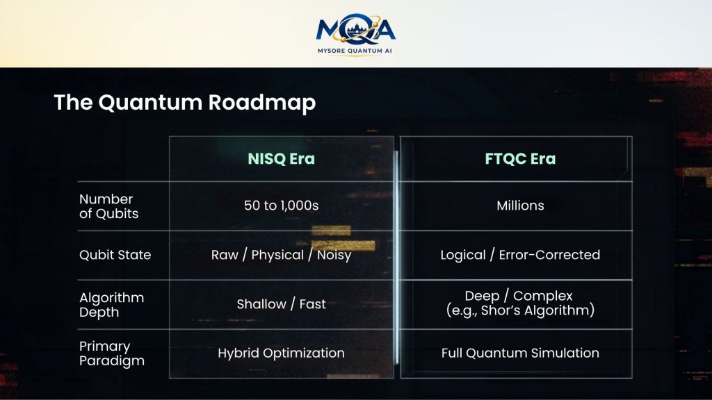
This refers to the number of physical qubits we can manipulate. Right now, we are in a zone ranging from roughly 50 to a few hundred (or low thousands) of qubits.
- Why “Intermediate”? It’s a very specific sweet spot. A quantum computer with 50 to 100 well-controlled qubits can perform operations so complex that even the world’s most powerful classical supercomputers cannot easily simulate them.
- However, it is still far too small for “fault-tolerant” quantum computing, which will require hundreds of thousands, if not millions, of physical qubits to run flawless, large-scale algorithms.
b. Noisy (The Problem)
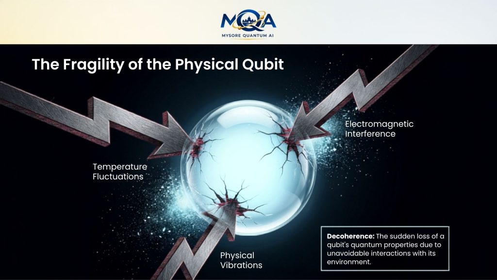
This is the defining challenge of our current era. Qubits are notoriously sensitive. They interact constantly with their environment with subtle temperature fluctuations, electromagnetic interference, or even physical vibrations can cause them to lose their quantum properties. This vulnerability is called decoherence.
Because of decoherence and imperfect quantum gates, errors creep into calculations very quickly. In a NISQ device, we do not have enough qubits to spare for Quantum Error Correction (QEC) a process that bundles thousands of fragile physical qubits together to create a single, perfectly protected logical qubit.
The Bottom Line: In the NISQ era, we have to run algorithms directly on the raw, unprotected, “noisy” physical qubits and just accept that errors will happen.
c. Why noise becomes a problem
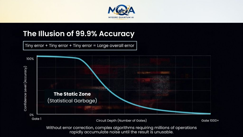
Suppose each gate operation is 99.9% accurate. That sounds excellent. But imagine executing:
- Gate 1 which is 99.9% accurate
- Gate 2 which is 99.9% accurate
- Gate 1000 which is 99.9% accurate
Small errors accumulate and after many operations:
Tiny error + Tiny error + Tiny error + … Large overall error
For complex algorithms requiring millions of operations, results may become unreliable.
The NISQ Dilemma: Scale vs. Noise
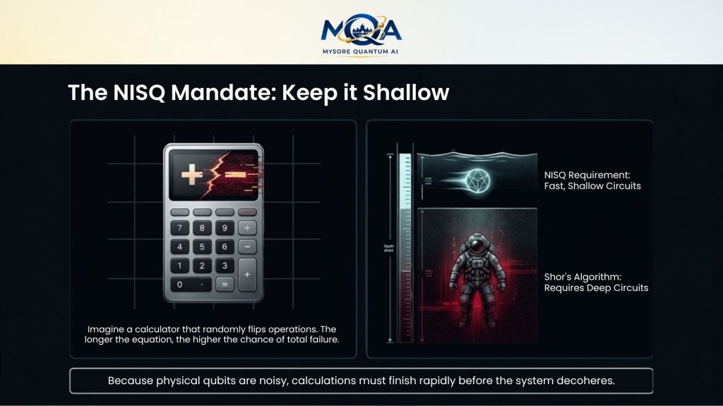
Think of a NISQ computer like a calculator that occasionally changes a + to a – at random, and the longer the equation you type, the more likely it is to make a mistake.
Because the qubits are noisy, we cannot run deep quantum circuits (algorithms with long sequences of logic gates). If a circuit is too deep, the cumulative noise completely overwhelms the calculation, turning the final output into pure statistical garbage. Therefore, NISQ algorithms must be shallow meaning they have to finish their calculations quickly before the qubits decohere.
What Can We Actually Do with NISQ?
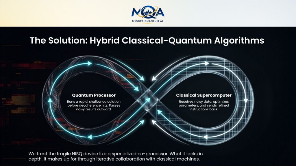
We can’t run ideal quantum algorithms like Shor’s Algorithm (for breaking modern encryption) on NISQ hardware which require millions of error-corrected qubits. Instead, researchers focus on Hybrid Classical-Quantum Algorithms.
These algorithms treat the NISQ processor like a specialized co-processor (similar to how a CPU offloads graphics tasks to a GPU). The quantum computer does a quick, shallow calculation, passes the noisy results to a classical computer, and the classical computer optimizes the parameters and sends a refined instruction back to the quantum computer.
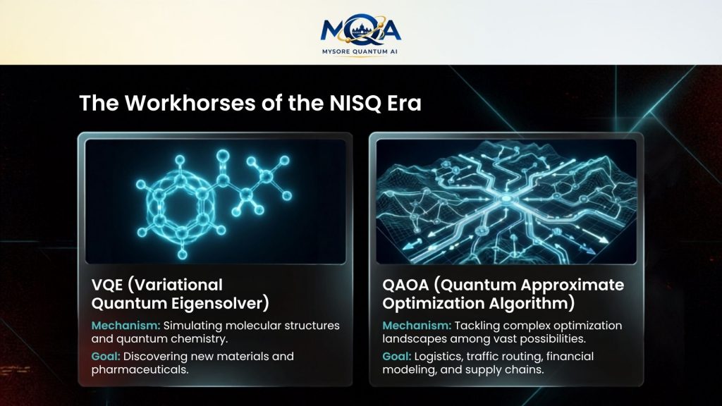
The two most prominent NISQ algorithms are:
- VQE (Variational Quantum Eigensolver): Used for simulating molecular structures and quantum chemistry to discover new materials or pharmaceuticals.
- QAOA (Quantum Approximate Optimization Algorithm): Used for tackling complex optimization problems, like logistics, supply chain routing, or financial modeling.
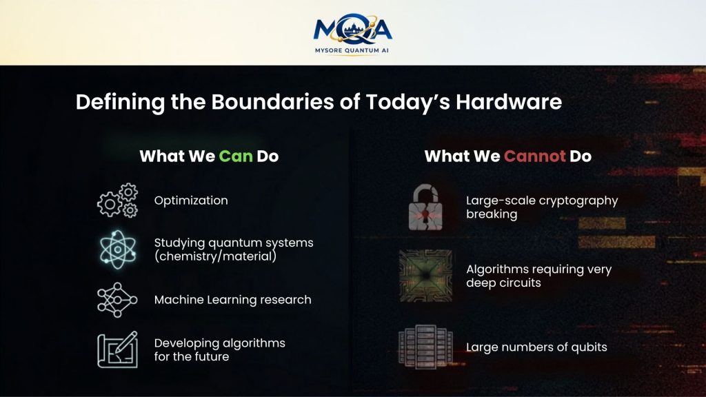
NISQ devices are already useful for research areas such as:
- Optimization: Finding efficient solutions among many possibilities.
Examples: Traffic routing, Scheduling and Supply chain problems
- Quantum simulation: Studying systems that are themselves quantum: Molecules, Materials and Chemical reactions
- Machine learning research: Exploring hybrid quantum-classical methods.
- Quantum algorithm development: Testing ideas for future large-scale systems.
What NISQ machines cannot yet do well
Current NISQ devices struggle with algorithms requiring Very deep circuits, Large numbers of qubits and Strong error correction
Examples include:
- Large-scale cryptography breaking
- General fault-tolerant quantum computation
- Very large scientific simulations
Where Are We Heading?
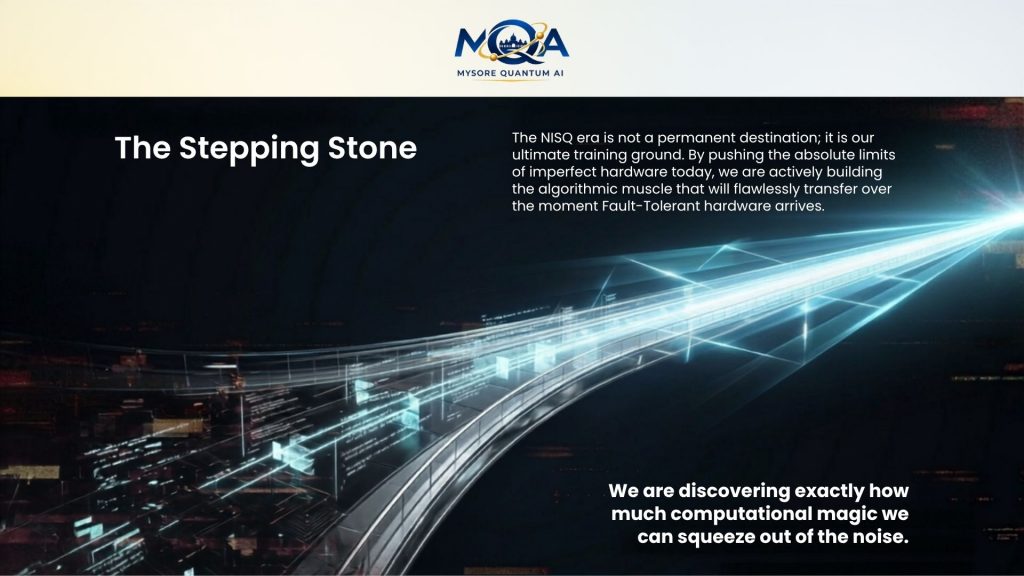
The NISQ era isn’t a permanent destination; it’s a critical stepping stone. The goal of companies like Google, IBM, and Rigetti is to transition from NISQ to Fault-Tolerant Quantum Computing (FTQC).
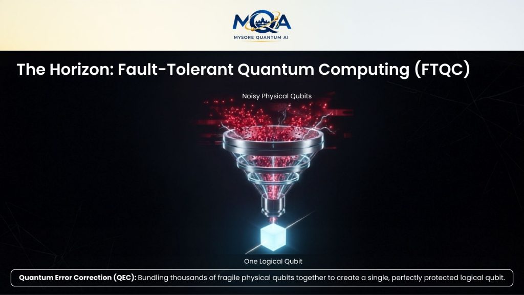
As physical qubit counts grow into the tens of thousands and error rates drop below critical thresholds, we will finally be able to implement full error correction
Until then, the NISQ era is our training ground, a time to push the limits of imperfect hardware and discover exactly how much computational magic we can squeeze out of the noise.