Grover’s Algorithm – Why It Speeds Up Search
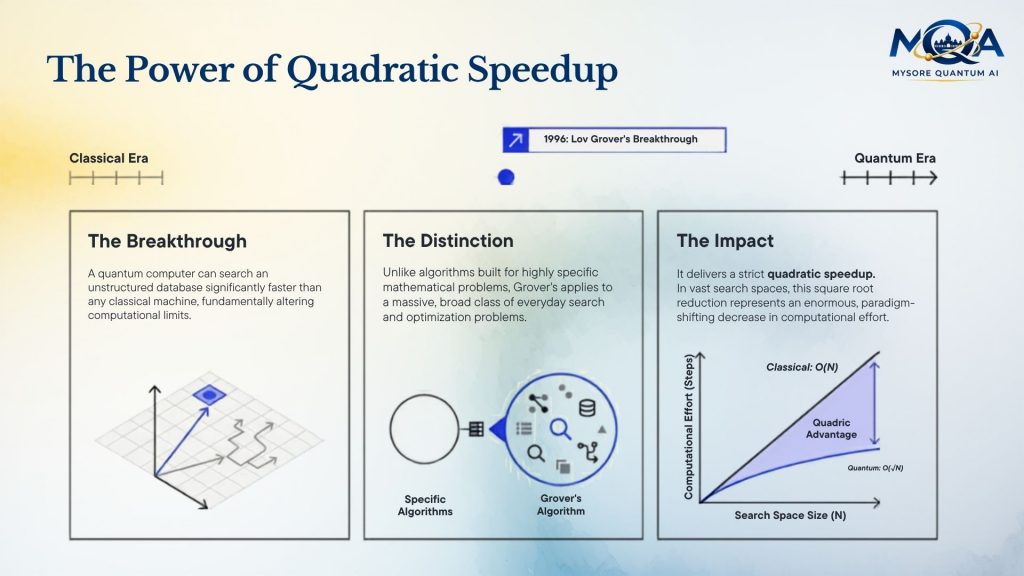
One of the most famous quantum algorithms is Grover’s Algorithm, developed by Lov Grover in 1996. It demonstrated that a quantum computer can search an unstructured database significantly faster than any classical computer.
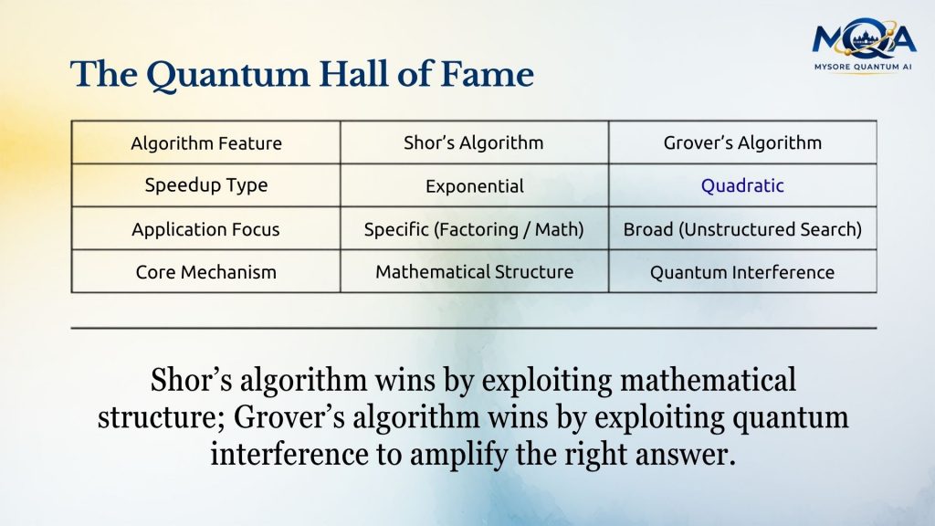
Unlike algorithms such as Peter Shor’s factoring algorithm, which provides an exponential speedup for specific problems, Grover’s algorithm provides a quadratic speedup for a very broad class of search problems.
Although quadratic may sound modest, for very large search spaces it represents an enormous reduction in computational effort.
The Search Problem
Imagine you have a database containing N items and only one item satisfies a condition: Find the record whose ID equals X.
The database is completely unstructured.
Classical Search
A classical computer has no choice but to check entries one by one.
On average: N/2 checks are required.
In the worst case: N
checks are required.
For example:
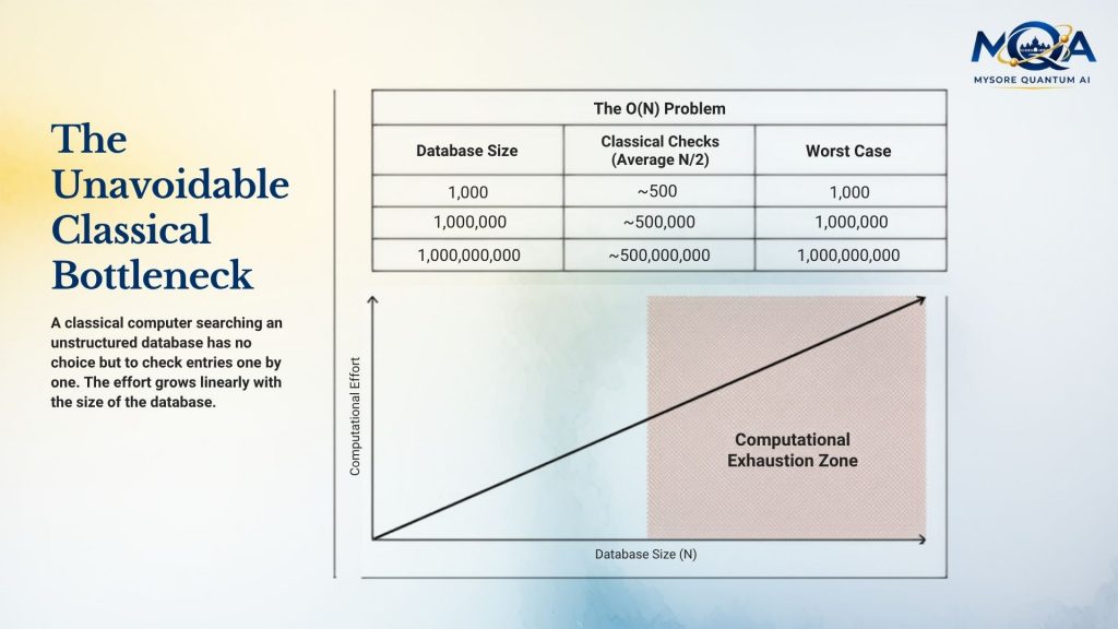
The effort grows linearly with the database size.
What Makes Quantum Search Different?
A quantum computer uses:
- Superposition
- Interference
- Amplitude amplification
Rather than checking entries individually, Grover’s algorithm increases the probability of the correct answer while decreasing the probabilities of all incorrect answers. Eventually, measurement reveals the desired item with high probability.
An Analogy: Finding One Correct Key
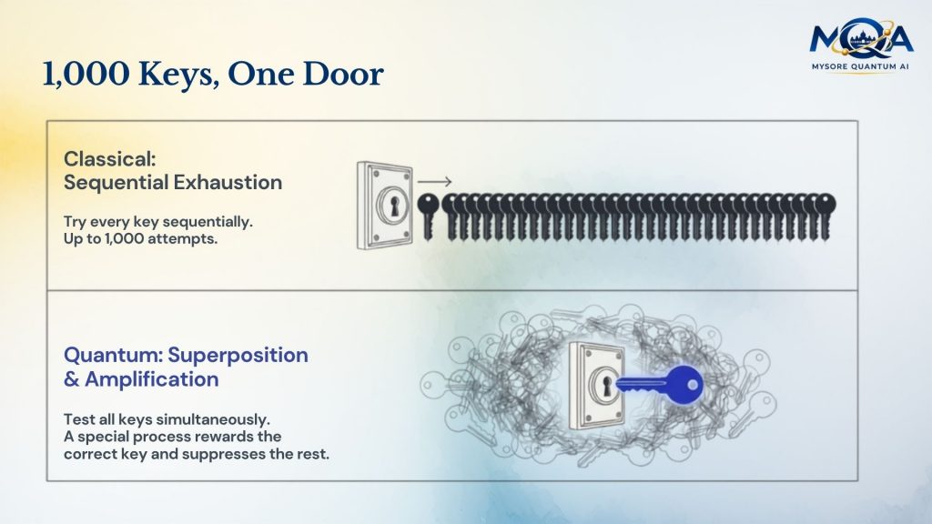
Suppose you have 1,000 keys and only one opens a door. In classical method all keys are tried one by one. In the worst case it would be 1,000 attempts.
Quantum Method
Imagine all keys are tested simultaneously in a quantum superposition.
Then a special process repeatedly:
- rewards the correct key
- suppresses incorrect keys
After enough repetitions, the correct key dominates.
When observed, the correct key appears with very high probability.
This rewarding process is called Amplitude Amplification.
Step 1: Create Superposition
Suppose we need to search among 4 possibilities.
The states are:
|00⟩, |01⟩, |10⟩, |11⟩
Initially:
|00⟩
Apply Hadamard gates:
H⊗n
Result:
½(|00⟩ + |01⟩ + |10⟩ + |11⟩)
The quantum computer now represents all possibilities simultaneously.
Visual Representation
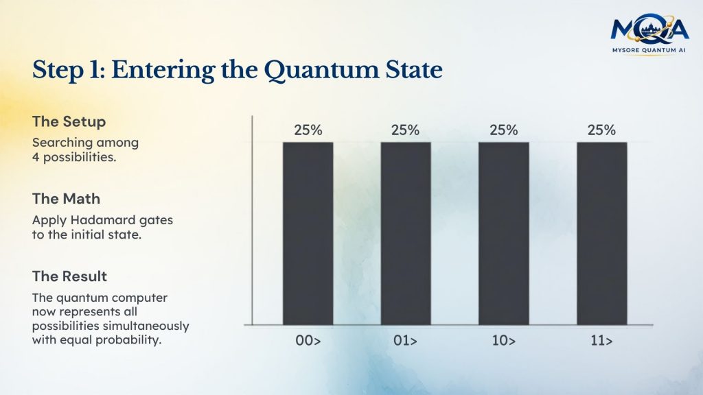
Every state has equal probability.
Step 2: Oracle Marks the Correct Answer
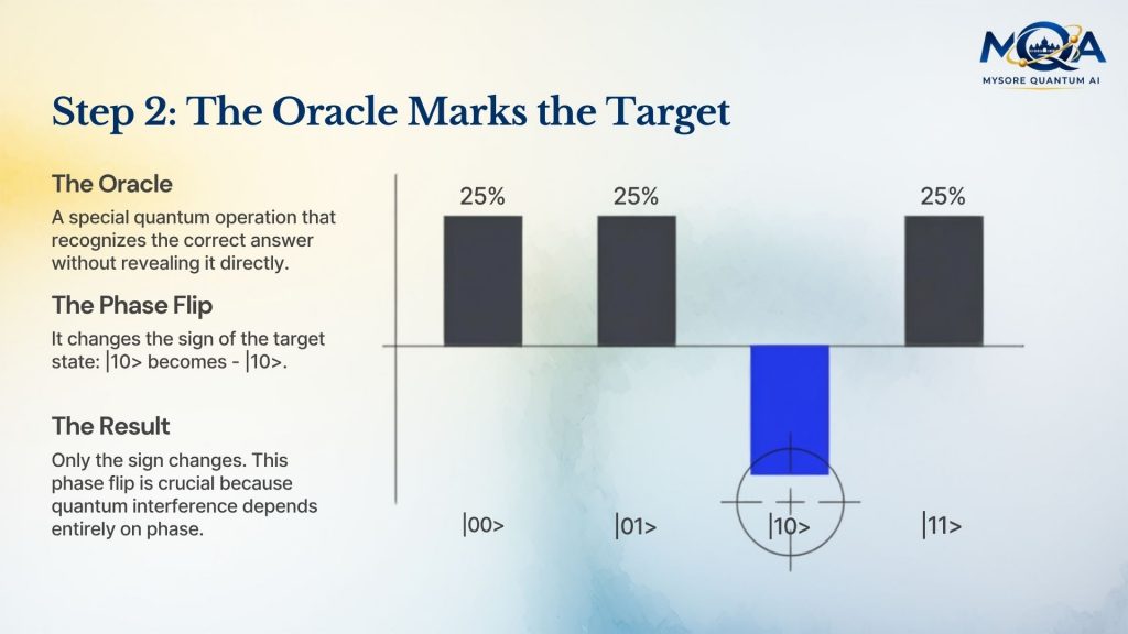
Assume: |10⟩ is the desired solution.
An Oracle is a special quantum operation that recognizes the correct answer.
It does not reveal the answer directly.
Instead it changes the phase:
∣10⟩ → −∣10⟩
Result:
½(|00⟩ + |01⟩ – |10⟩ + |11⟩)
Only the sign changes.
This phase flip is crucial because interference depends on phase.
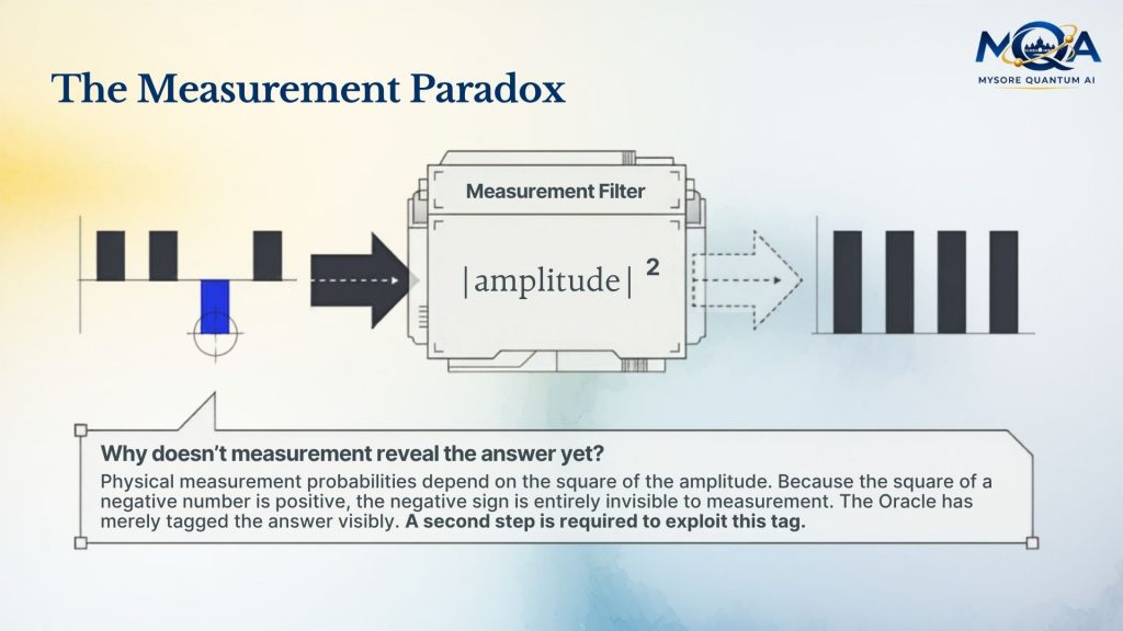
Why Doesn’t Measurement Reveal the Answer Yet?
Because probabilities depend on:
|amplitude|²
and
(1/2)² = (□ -1/2)²
The negative sign is invisible to measurement. The oracle merely tags the correct answer. A second step is needed to make use of that tag.
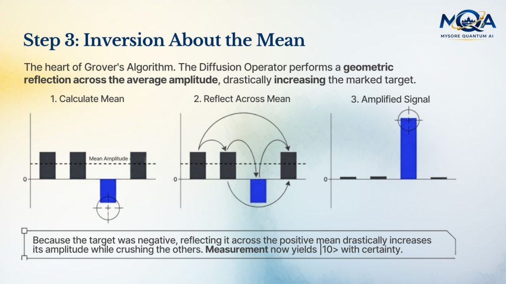
Step 3: Diffusion Operator
This is often called Inversion About the Mean. It is the heart of Grover’s algorithm.
The diffusion operator performs a geometric transformation that:
- increases the marked state’s amplitude
- decreases the others
Before Diffusion
0.5
0.5
-0.5 ← marked
0.5
Mean amplitude: 0.25
Reflection about the mean causes:
0
0
1
0
The marked state now has all the probability.
Measurement gives: |10⟩ with certainty.
The Amplification Cycle
The sequence:
- Oracle
- Diffusion
is called a Grover Iteration. Each iteration rotates the quantum state toward the solution.
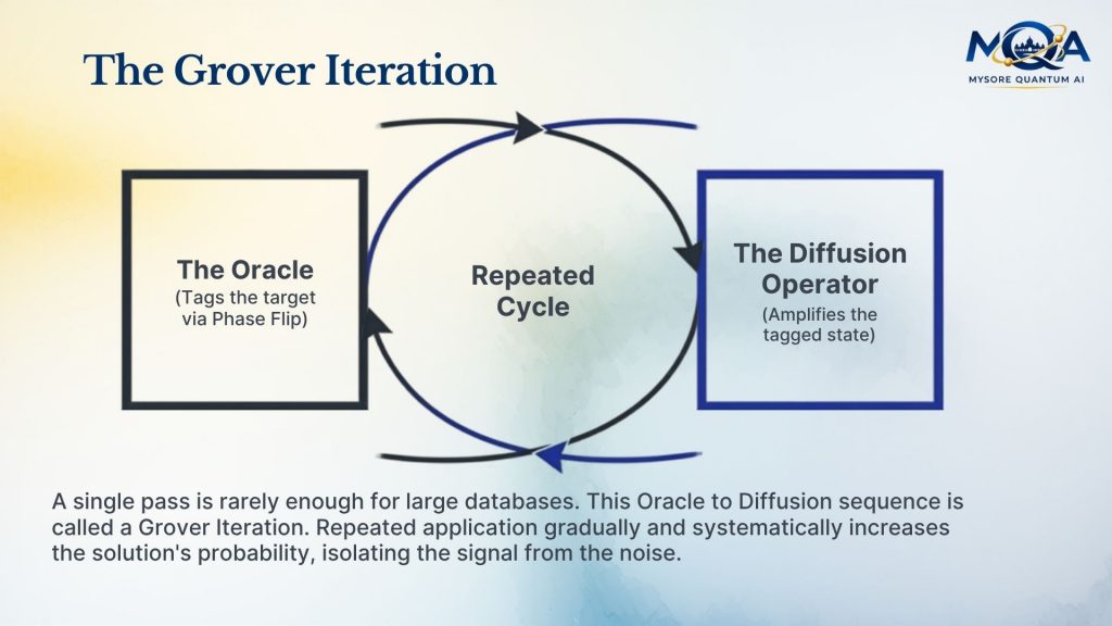
Repeated application gradually increases the solution probability.
Geometric Interpretation
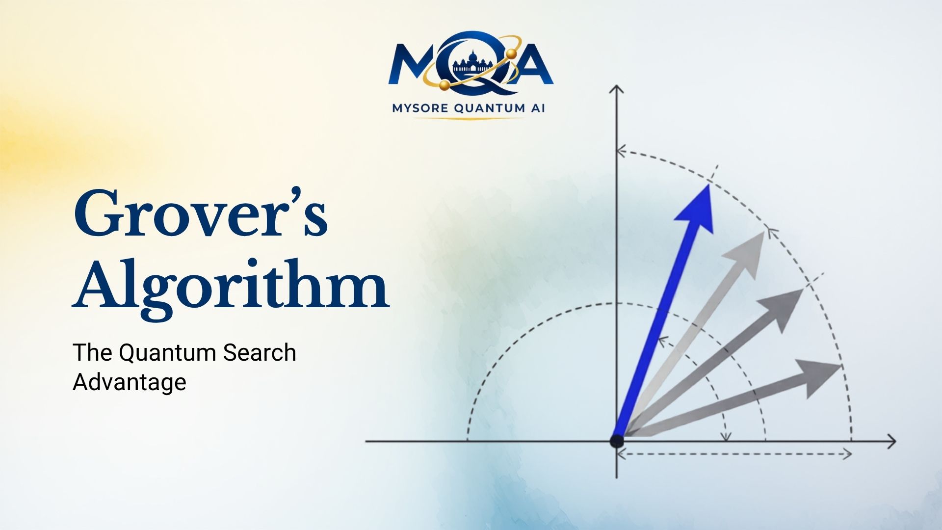
A beautiful way to understand Grover’s algorithm is as a rotation. The quantum state exists in a two-dimensional space:
Solution Direction
|w⟩
Non-Solution Direction
|r⟩
Initially:
|s⟩
is mostly aligned with the non-solution direction.
The oracle and diffusion operator act like mirrors.
Two reflections produce a rotation.
Each Grover iteration rotates the state closer to:
|w⟩
Eventually nearly all amplitude points toward the solution.
Visualizing the Rotation
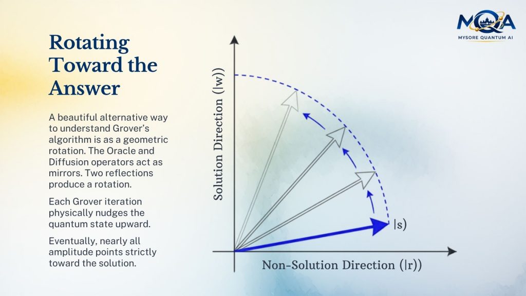
Each iteration nudges the state upward toward the solution axis.
How Many Iterations Are Needed?
This is where the speedup appears. For a search space of size:
Grover requires approximately: (π/4) √N iterations.
Comparison
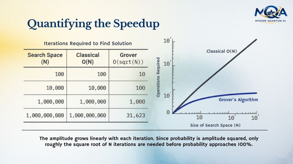
The improvement grows as the search space increases.
Why Is This Faster?
Classically: 0(N)
Quantumly: 0(√N)
The reason is that amplitude grows linearly with each Grover iteration.
Since probability equals:
(amplitude)²
only about: √N iterations are needed before the probability approaches 1. This relationship between amplitude and probability is the source of the quadratic speedup.
Is Grover Searching Everything Simultaneously?
A common misconception is: The quantum computer checks all database entries at once but not exactly.
The speedup comes from:
- superposition
- phase marking
- interference
- amplitude amplification
The algorithm does not magically read every item.
Instead, it manipulates probability amplitudes so that the correct answer becomes increasingly likely.
Multiple Solutions
Suppose there are: valid answers among
items. Grover’s algorithm requires:
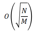
iterations. More valid solutions mean fewer iterations.
Real-World Applications
Grover’s algorithm applies whenever a problem can be framed as: Find an input that satisfies a condition.
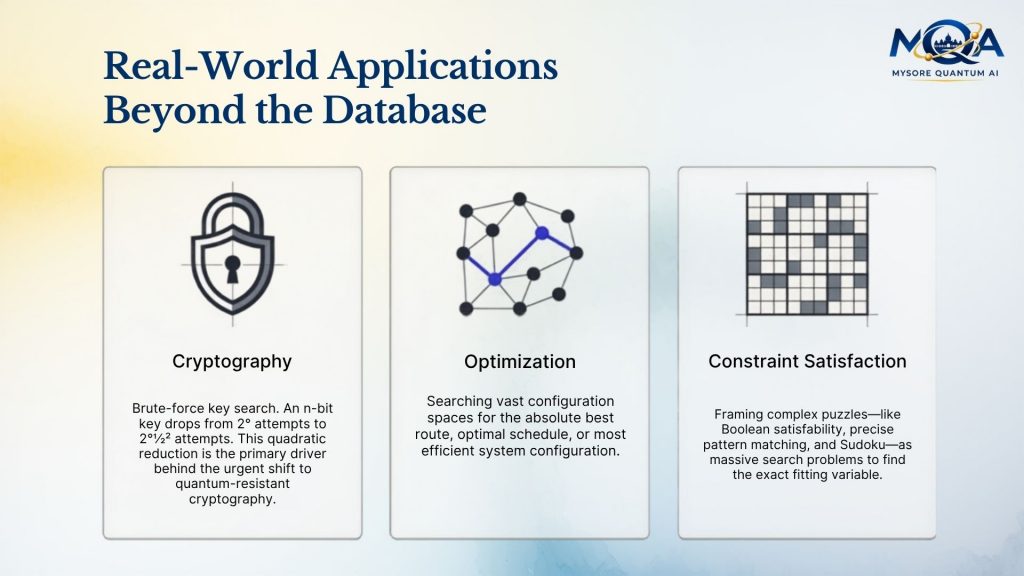
For an n-bit key:
Classical: n² attempts.
Grover: 2 n/2 attempts.
This is why quantum-resistant cryptography is important.
Optimization
Searching for:
- best route
- best schedule
- best configuration
among many possibilities.
Constraint Satisfaction
Examples:
- Sudoku solving
- Boolean satisfiability
- Pattern matching
when formulated as search problems.
Limitations
Grover’s algorithm is powerful, but not magic.
It Does Not Give Exponential Speedup
The improvement is:
(0)N ->0(√N)
which is quadratic.
Requires an Oracle
The algorithm assumes a function exists that can verify whether a candidate is correct.
Building the oracle may itself be difficult.
Error Sensitivity
Large-scale Grover search requires:
- many qubits
- low error rates
- fault-tolerant quantum computers
Current NISQ devices are generally too small to outperform classical systems on large search problems.
Intuition in One Sentence
Grover’s algorithm speeds up search by repeatedly using quantum interference to increase the probability amplitude of correct answers and decrease the amplitudes of incorrect ones, allowing a solution to be found in roughly √N steps instead of N steps.
Key Takeaways
- Grover’s algorithm searches an unstructured space of N possibilities.
- Classical search requires O(N) checks.
- Quantum search requires O(√N) oracle calls.
- The algorithm relies on:
- Superposition
- Oracle phase marking
- Interference
- Amplitude amplification
- The oracle tags the correct answer with a phase flip.
- The diffusion operator amplifies the tagged state’s amplitude.
- Repeated Grover iterations rotate the quantum state toward the solution.
- The quadratic speedup is provably optimal for unstructured search.
- Grover’s algorithm impacts cryptography, optimization, and search problems.
- It remains one of the most important demonstrations of quantum advantage in algorithm design.
A useful way to remember Grover’s algorithm is:
Shor’s algorithm wins by exploiting mathematical structure; Grover’s algorithm wins by exploiting quantum interference to amplify the right answer.